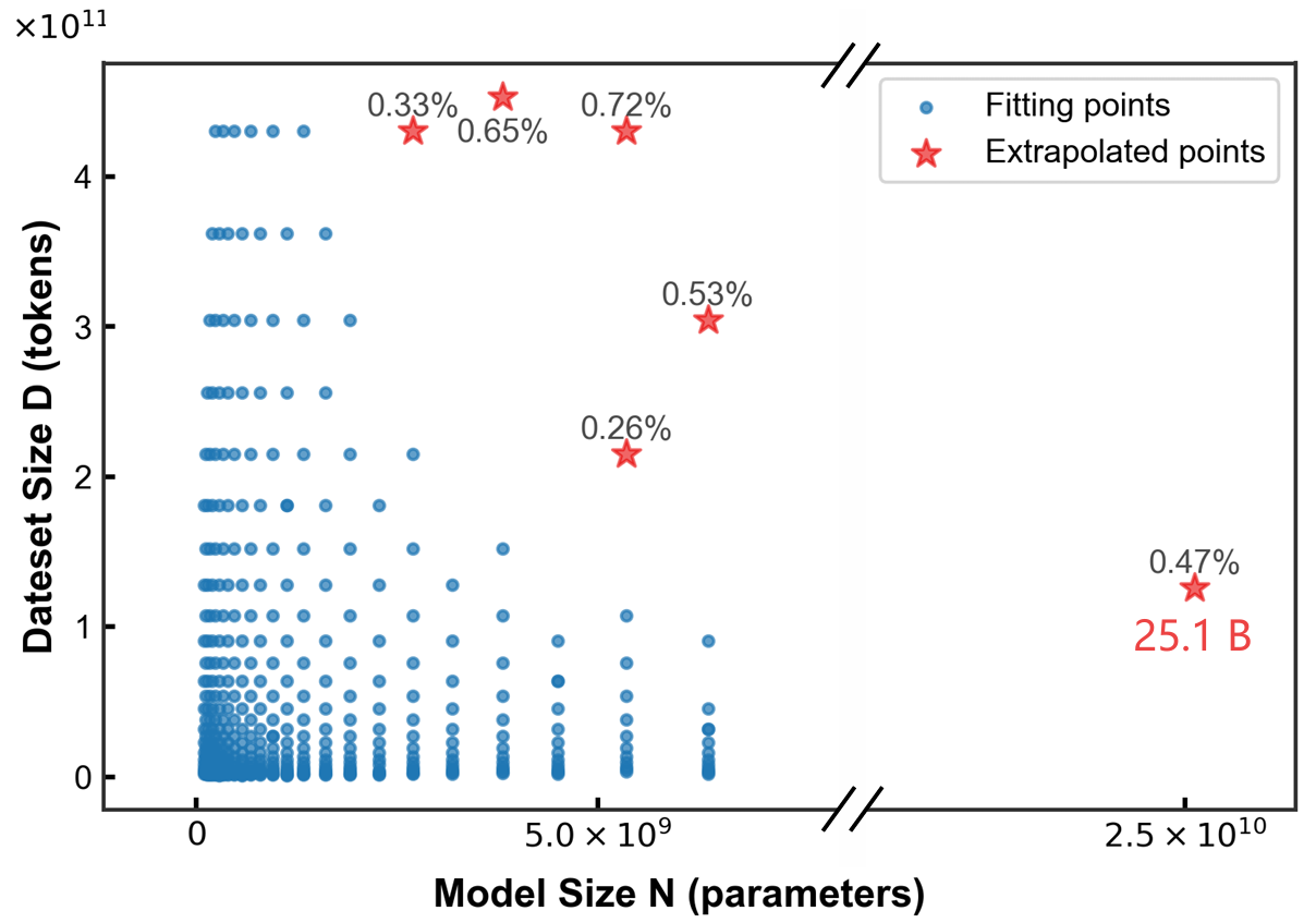
We present Farseer, a novel and unified scaling law that offers unprecedented predictive accuracy for Large Language Models (LLMs). Our findings demonstrate remarkable extrapolation capabilities, reducing prediction error by 433% compared to Chinchilla's law and enabling highly accurate forecasts of large-scale performance from small-scale experiments.
This research represents a significant computational investment, utilizing approximately 3 million NVIDIA H100 GPU hours to train a comprehensive suite of nearly 1,000 LLMs from scratch. By systematically constructing the model loss surface L(N,D), Farseer provides a robust and generalizable framework that bridges the critical scaling gap between experimentation and production.
To support reproducibility and advance the field of LLM pre-training, we will progressively release our full dataset of loss measurements and checkpoints.
Step Law demonstrates that the optimal batch size $B(D)$ exhibits a primary dependence on dataset size $D$, while the optimal learning rate $\eta(N, D)$ manifests a joint dependence on both model parameters $N$ and dataset size $D$.
Farseer's prediction error consistently decreases as the amount of fitting data increases, demonstrating strong robustness. It also exhibits excellent generalization across different data distributions.
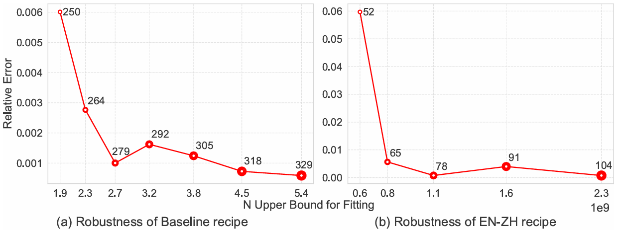
Left Figure: The prediction error for Farseer decreases significantly as the amount of fitting data increases. For instance, when the upper bound for model size in the fitting data is expanded from 1.9B to 5.4B parameters, the relative prediction error for a 6.4B model drops from 0.6% to 0.058%, showcasing its robustness to data quantity. Right Figure: On bilingual English-Chinese (EN-ZH) data, as the amount of fitting data increases, the prediction error for a 3.2B model converges to 0.076%. This indicates its generalization capability across different data distributions, effectively capturing the scaling patterns of cross-lingual data.
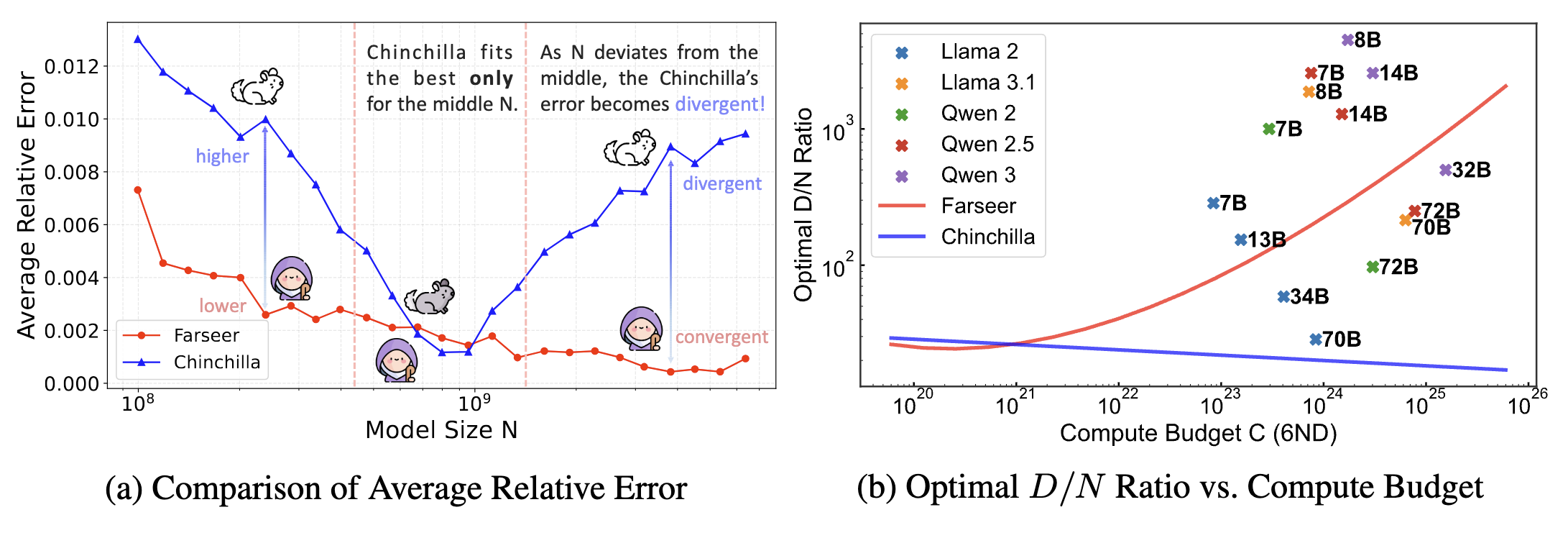
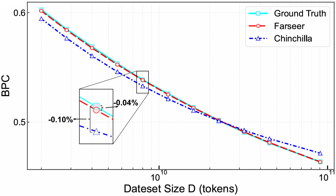
Farseer's average relative error is just 0.50%, whereas the Chinchilla scaling law exhibits an average relative error of 2.68%, a 433% increase.
Besides, our research findings reveal that this scaling law not only applies to dense models but also generalizes effectively to MoE models with varying sparsity levels, demonstrating robust generalization capabilities.
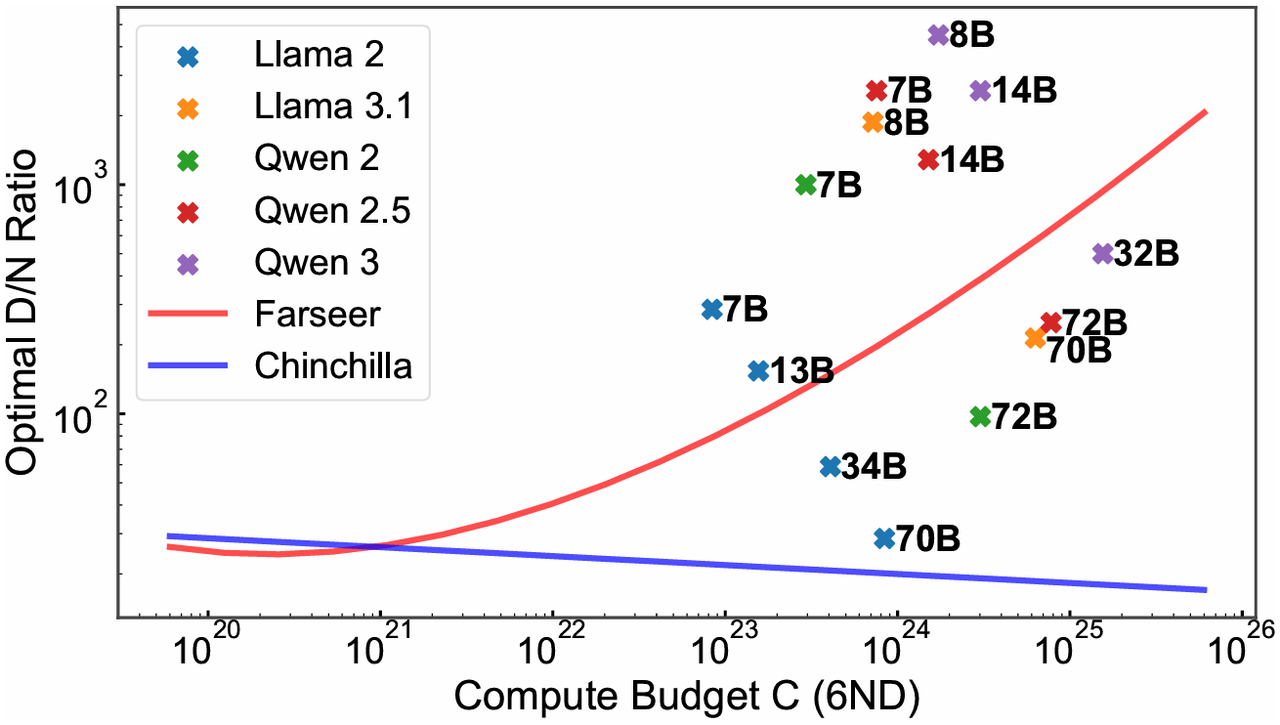
Under the condition C≈6ND, Chinchilla recommends a fixed D/N≈20, which is only applicable for medium compute budgets ($10^20−10^21FLOPs). Farseer,however, predict that the optimal D/N ratio continuously increases with the compute budget, which is fundamentally consistent with the training configurations of large models like Llama 3.1 and Qwen 3.
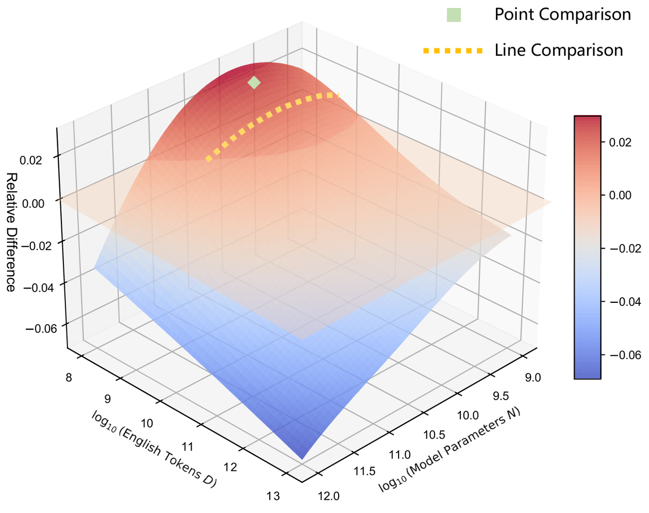
Regions above the plane indicate that the 50\% English mixture yields lower error, while regions below favor the 85\% mixture. Green squares denote individual point comparison experiments at specific \((N,D)\) coordinates, and the yellow line connects several such points for a line comparison. Although these smaller scale analyses can suggest one mixture is better, the surface comparison reveals how those conclusions can reverse at larger scales. \textit{Farseer}\text{'}s exhibits power for low-cost, high-fidelity extrapolation across any two training recipes or model designs.
@misc{li2025predictablescalei,
  title    = {Predictable Scale: Part I -- Optimal Hyperparameter Scaling Law in Large Language Model Pretraining},
  author   = {Houyi Li and Wenzheng Zheng and Jingcheng Hu and Qiufeng Wang and Hanshan Zhang and Zili Wang and Shijie Xuyang and Yuantao Fan and Shuigeng Zhou and Xiangyu Zhang and Daxin Jiang},
  year     = {2025},
  eprint   = {2503.04715},
  archivePrefix = {arXiv},
  primaryClass  = {cs.LG},
  url      = {https://arxiv.org/abs/2503.04715},
}